![]()
|
|
|
|
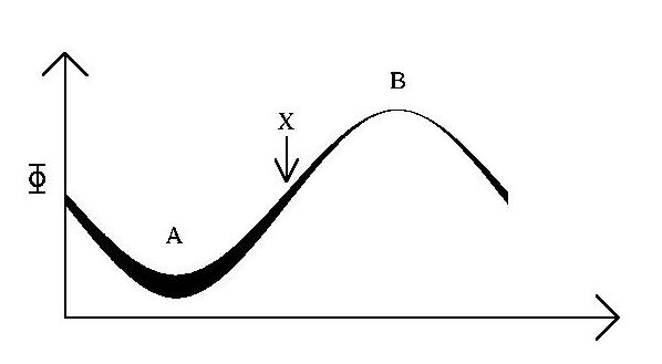
Acoustic Oscillations and Apparent Temperature Variations The ebb and flow of the plasma during the acoustic oscillations can be better understood if gravity and photon pressure are combined into a single restoring force. This can be done by considering how gravitational redshifts affect the apparent temperature of a source. Imagine an object at some intrinsic temperature (the temperature an observer located at the source would report) is sitting at the bottom of a potential well. As the thermal radiation from the source climbs out of the potential well, the photons are redshifted such that the source appears to be cooler than its intrinsic temperature. Conversely, a source located at a potential maxima will appear warmer than its intrinsic temperature when the photons blueshift as they fall down the slope in the potential. Note that while the apparent temperature of a source depends on the location of the observer, the difference in the apparent temperatures of two sources is the same for all observers.
Figure 1.7: Apparent temperature fluctuations. A section of the plasma is shown with a sinusoidal variation in the (intrinsic) temperature of the plasma (illustrated by the varying thickness of the line) and the gravitational potential (indicated by the varying height of the line). For the observer at point X the radiation emitted from point A is redshifted, causing the plasma to appear colder, while the radiation emitted from point B is blueshifted, thus appearing warmer. Therefore the observer at X sees an apparent temperature difference between points A and B that is smaller than the intrinsic temperature difference. In the primordial plasma, overdense regions were both warmer than underdense regions (by the ideal gas law) and at lower gravitational potentials. In this situation, the gravitational redshifts cause the apparent temperature variations to be smaller than the intrinsic temperature variations (see Figure 1.7). In principle, the gravitational redshifts could balance the intrinsic temperature variations exactly, so that there would be no variations in the apparent temperature. In this perfectly balanced case, the plasma would appear homogeneous, and there could be no net force acting to redistribute the plasma. If the variations in the gravitational potential were slightly smaller (relative to the intrinsic temperature variations), not only would overdense regions appear warmer than underdense regions, but also the net gravitational force would be slightly weaker than the force due to photon pressure (material would tend to move out of overdense regions into underdense regions). Conversely, slightly larger variations in the gravitational potential would result in the overdense regions appearing cooler than underdense regions and the gravitational force overcoming the pressure force (material would tend to move out of underdense regions into overdense regions). In both of these cases material moves from apparently warmer regions to apparently cooler ones. Therefore the plasma dynamics can be described in terms of a single restoring force acting to minimize the apparent temperature variations. The initial conditions laid down by inflation were such that each mode originally had a nonzero apparent temperature variation. Consequently, once the horizon scale became larger than the wavelength of a mode, the size of the apparent temperature variation in that mode oscillated about zero like a harmonic oscillator.
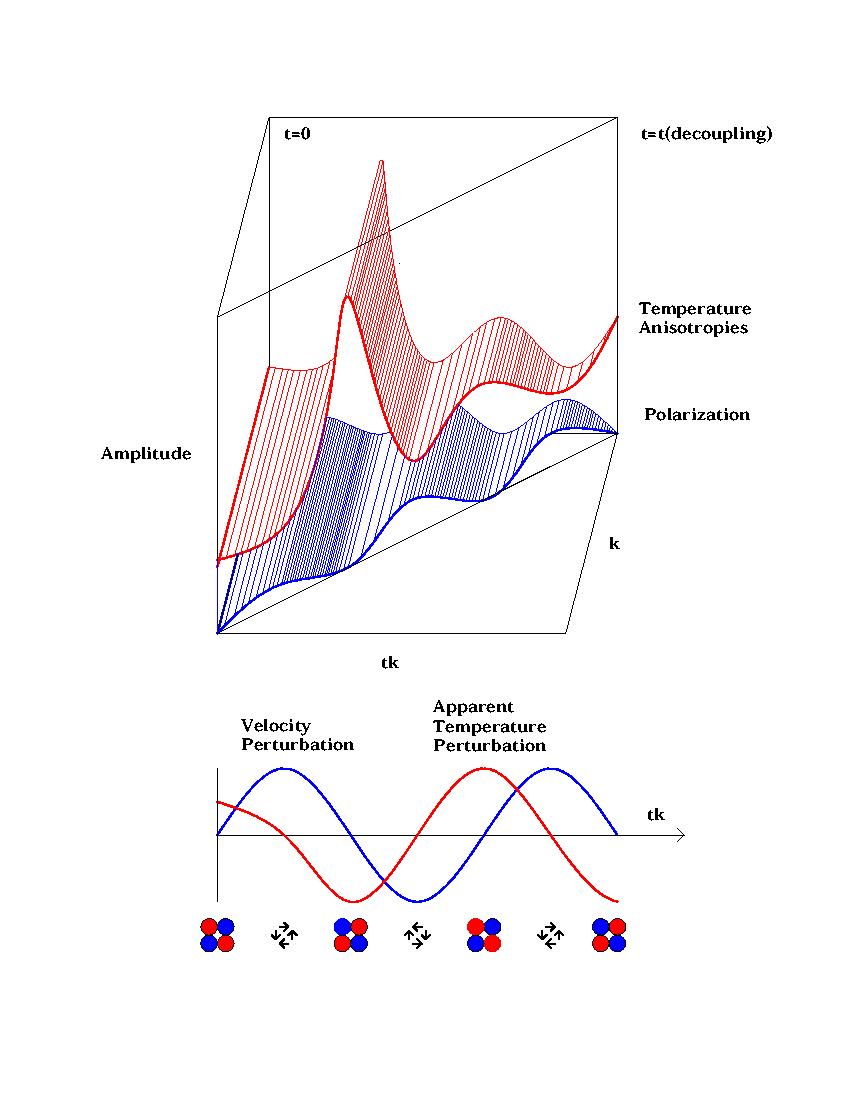
Figure 1.8: The evolution of structure in the CMB. At the bottom of this figure is a graph that shows the evolution of the amplitudes of the apparent temperature and velocity perturbations of a single mode as a function of tk, where k is the mode wavenumber and t is cosmic time (The ratio of mode wavelength to horizon scale, which determines the evolution of the oscillation, is directly proportional to tk ). The size of the velocity and temperature perturbations oscillate about zero as material ebbs and flows between apparently hot and cold spots, as shown by the icons at the bottom of the plot. The upper part of the figure shows a graph with the axes, k,tk and the rms of the variations. The left side of this box corresponds to t=0, so on this wall of the box the initial conditions are displayed. The polarization is zero here because the velocity perturbations were initially zero, while the temperature fluctuations have a flat power spectrum due to the assumption of scale invariant initial conditions. Each of the modes evolved as a function of tk as shown in the lower part of the figure, indicated by the rippled surfaces (which are positive definite because the rms of the variations are shown). Since the lower axes are k and tk, a single moment of time corresponds to a vertical plane intersecting the z-axis, and increasing time corresponds to rotating the plane. The plane which forms the edge of the surfaces corresponds to the epoch of decoupling. On this plane, modes with larger k (smaller wavelength) correspond to higher values of tk (a later point in the oscillations), so that the power spectrum at decoupling recapitulates the evolution of a single mode. These power spectra are in terms of length scales: the angular power spectra of the CMB have similar shapes because l approximately equals k. The Origin of Cosmological Polarization The Structure of Cosmological Polarization Power Spectra and the Structure of CMB Anisotropies Initial Conditions and Inflation The Evolution of Perturbations and Acoustic Oscillations Acoustic Oscillations and Apparent Temperature Variations |
|
|